How to describe bivariate data

Association between explanatory and outcome variables, causation and covariation

One of the main goals of statistical analysis is to study the association between variables.

There is an association between two variables if one variable tends to display specific values when the other one changes. For example, let’s take into account a variable called “Response to treatment” (displaying the values: “Worsened/Stable/Improved”) and a variable called “Treatment” (displaying the values “Treatment A” and “Treatment B”). If treatment B is placebo, it is likely that individuals receiving treatment A will be mostly improved compared to individuals receiving treatment B. In this case, there is an association between the variables “Response to treatment” and “Treatment” because the proportion of individuals who are responding to treatment changes along with different type of treatments.

Usually, when an association between two variables is analyzed (the so called “Bivariate analysis”), one variable is defined as the “Outcome variable” and its different values are compared based on the different values displayed by the other variable, which is defined as the “Explanatory variable”. The values displayed by the explanatory variable define a subset of groups that will be compared; differences among different groups will be assessed based on the values displayed by the outcome variable.

Bivariate Analysis, as outlined above, allows an assessment of how the value of the outcome variable depends on (or is explained by) the values displayed by the explanatory variable (1). For example, if we try to compare gender and income, the latter is the outcome variable while the former is the explanatory variable; income, in fact, may be influenced by gender but gender many not depend on the income.

Two types of bivariate analysis may be defined, each with definite features and properties (2):

• Dependence analysis:
• Describes how the outcome variable changes when the independent or explanatory variable changes. The bond between the two variables is unidirectional or asymmetrical;
• Logic dependence: there is a cause and effect relationship between two or more variables;
• Logic independence: there isn’t any cause and effect relationship between the variables that are considered.
• Inter-dependence analysis:
• Describes the interaction between the values displayed by two variables (bidirectional or symmetrical bond);
• A relationship of dependence is not possible;
• A dependent character may not be found.

A causal explanation is one of the key goals of scientific research. When we define a cause and effect relationship, we are referring to the existence of a bond between two events, so that the occurrence of one specific event is the direct consequence of the occurrence of another event (or a group of events). A simple empirical relationship between two events does not necessarily define the concept of causation. In fact, “Co-variation” does not mean “Causation”.

Covariation (correlation or association) means that we are just looking at the fact that two variables called X and Y present concurrent variations: when one changes the other changes too. Causation means that the hypothesis that the variation of X is determining a variation of Y is true.

Attributing a causal bond to any relationship between two variables is actually a weak attribution. Reality is—per se—a “multi variated” world, and every phenomenon is related with an infinity of other phenomena that interact and link with each other. In fact, multivariate analysis helps finding a better approximation of the reality and therefore represents the ultimate goal of data analysis. Nevertheless, univariate analysis and bivariate analysis are a basic and necessary step before proceeding to more complex multivariate analysis.

Unfortunately, there is no perfect statistical methodology available to define the true direction of causality. Other important available tools are the researchers’ experience and the ability to appropriately recognize the nature of the variables and the different types of studies, from cohort studies to randomized controlled studies and systematic reviews.

Therefore, bivariate statistics are used to analyze two variables simultaneously. Many studies are performed to analyze how the value of an outcome variable may change based on the modifications of an explanatory variable. The methodology used in these cases depends on the type of variable that is being considered:

• Qualitative nominal variables (in these cases we will be dealing with “Association”);
• Qualitative ordinal variables (in these cases we will be dealing with “Co-graduation”);
• Quantitative variables (in these cases we will be dealing with “Correlation”).

Qualitative bivariate data

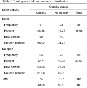
Given two categorical variables, a contingency table shows how many observations are recorded for all the different combinations of the values of each variable. It allows to observe how the values of a given outcome variable are contingent to the categories of the explanatory variable. Using this model, a first synthetic analysis maybe given by the marginal, conditional or conjugate distribution (3-5). The marginal distributions correspond to the totals of the rows and of the columns of the table; conditional distributions correspond to all the percentages of the outcome variable calculated within the categories of the explanatory variable; conjugate distribution is given by a single group of percentages for all the cells of the table, divided by the overall size of the sample (Table 1).

Table 1 Contingency table and conjugate distribution
Full table

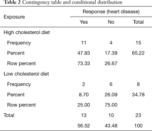
When it is possible to distinguish between an outcome and an explanatory variable, conditional distributions are much more informative than conjugate distributions. Using a contingency table to analyze the relationship between two categorical variables, we must distinguish between row percentages and column percentages. This choice is performed based on the position that a given dependent variable is holding. The column percentage is chosen if we want to analyze the influence that the variable placed in column has on the variable in the row; the row percentage is chosen when we want to assess the influence that the row variable has on the variable in the column (Table 2).

Table 2 Contingency table and conditional distribution
Full table

The principle of assigning a percentage to the independent variable is our best choice when our aim is to study the causal relationship between the independent and the dependent variable. In other situations, it might be useful to calculate the percentages in the opposite directions or in both ways. This last approach is usually adopted when it is not clearly possible to distinguish between a dependent and an independent variable (Table 1).

There are statistical techniques that are able to measure the strength of the relationship between the variables of the study, and these techniques may contribute to reduce the subjectivity of the analysis. As previously mentioned, we may distinguish measures of association for nominal variables and co-graduation measures for ordinal variables. Among these, the most common are:

• Association: chi-squared test (χ²), Fisher’s exact test;
• Co-graduation: Kendall’s tau-c (τc), Kruskal’s gamma (ϒ), Somers’D.

Specific interest is provided by the “2×2” tables, which are tables where both variables are dichotomous. In this type of tables we may calculate other measures of association, for example:

• d = difference between proportions;
• OR (ψ) = odds ratio;
• RR = relative risk.

All these measures are used after verification of all the basic assumptions of the standard practice of calculation, and are based on the type of study that we need to perform (retrospective/prospective).

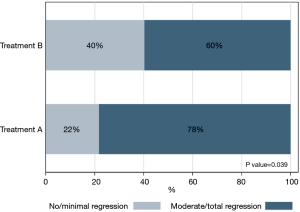
Sometimes it may be useful to graphically present the relationship between two categorical variables. In order to do this, there are tools that are used to describe the frequency distributions of univariate variables: these tools are bar charts (Figure 1).

Figure 1 Example of a bar chart.

Quantitative bivariate data

In case of two quantitative variables, the most relevant technique for bivariate analysis is correlation analysis and simple linear regression.

Using the latter methodology, it is possible to understand how the independent variable may influence the dependent variable or, more specifically, it is possible to assess the intensity of the effect of the independent variable on the dependent variable (6).

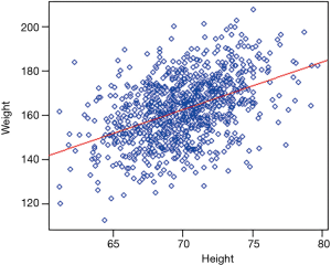
The first step in the construction of a model for bivariate analysis with quantitative variables is to display a graphical representation of the relationship by using a scatterplot (or dispersion diagram), which is able to show visually how the two variates co-variate (= variate together) in a linear or non-linear fashion (Figure 2). This diagram is able to show us the shape of the relationship but cannot measure the intensity of the causal effect.

Figure 2 Example of a scatterplot box.

The second step is measuring the strength of the linear association bond between the variables, by using the correlation analysis. This is expressed by a number between −1 and +1 and it shows if the values of the two variables tend to increase or decrease simultaneously (positive correlation) or if one increases and the other decreases (negative correlation) Figure 3.

Figure 3 Examples of linear correlation.

What is even more interesting is to perform a quantitative assessment of the variation of one of the two variables (chosen as dependent variable) compared to the changes of the second variable (independent variable), using a mathematical equation. This equation, if the linear profile of the relationship is confirmed, is the basis of simple linear regression: a mathematical function describing how the mean value of the outcome variable changes according to the modifications of the explanatory variable.

Comparing groups with bivariate analysis

The comparison of two populations displaying, for example, a quantitative and a qualitative variable may also be performed using bivariate analysis (7). In this case, it is particularly useful to compare the mean values of the continuous variable to the different categories of the other variable, using the plot box graph as a preliminary analysis.

Specific bivariate statistical models are available for the cases where a given variable is analyzed according to different categories of a further variable, for example the analysis of variance (ANOVA).

Take home messages

• Bivariate statistics are used in research in order to analyze two variables simultaneously;
• Real world phenomena such as many topics of scientific research are usually complex and multi-variate. Bivariate analysis is a mandatory step to describe the relationships between the observed variables;
• Many studies have the aim of analyzing how the values of a dependent variable may vary based on the modification of an explanatory variable (asymmetrical analysis);
• Bivariate statistical analysis, and, accordingly, the strength of the relationship between the observed variables, may change based on the type of variable that is observed (qualitative or quantitative).

Acknowledgements

None.

Footnote

Conflicts of Interest: The authors have no conflicts of interest to declare.

References

1. Agresti A. Categorical Data Analysis, 1th ed. Wiley, 2002.
2. Agresti A, Finlay B. Statistical Methods for the Social Science, 4th ed. Pearson, 2009.
3. Corbetta P, Gasperoni G, Pisati M. Statistica per la Ricerca Sociale, Il Mulino, 2001.
4. Vittinghoff E, Glidden DV, Shboski SC, et al. Regression Methods in Biostatistics, 2th, Springer, 2012.
5. Afifi A, May S, Clark VA. Practical Multivariate Analysis, 5th. Chapman Hall/CRC, 2011.
6. Collet D. Modelling binary data, 2th. Chapman Hall/CRC, 2003.
7. Available online: https://www.mathsisfun.com