A brief introduction to probability

Probability

A simple clinical vignette may help introducing the concept of probability.

In a clinical study, patients with claudicatio intermittens who received treatment “A” walked an average of 472 m, while patients who received treatment “B” walked 405 m. Given the difference of 67 m in favor of treatment “A”, is it possible to conclude that, based on this study, treatment “A” is better than treatment “B”? And, based on this assumption, should the doctor administer treatment “A” to his next patient with claudicatio intermittens?

The first question is a typical question involving the concept of statistical inference and, precisely, is: “what is the conclusion that we may draw from our study?”

The second question is a typical question about decision-making: what is the rationale for preferring a specific treatment over another, based on the information available in the study and other information coming from previous studies?

The answers to both questions may be provided with just a limited amount of uncertainty, although uncertainty may vary in different circumstances. If the degree of uncertainty is low, the conclusions will be strong and the decision based on the available knowledge (or evidence) will be almost certain. If the degree of uncertainty is high, the conclusions will be poor and the decision will not be based on evidence but will be only based on personal experience, instinct, or will be left to chance.

It is therefore very important to measure the degree of uncertainty, and the theory of probability provides us with the appropriate tools to do so. Probability may also be defined as the “logic of the possible” or the “logic of the uncertain”, because it has to deal with hypotheses that may not be associated with a completely true or false attestation, but just with a “possible” attestation. For example, “tomorrow will rain” is neither a true or false hypothesis, but it is only possible. For all the hypotheses that have to deal with uncertainty, the theory of probability will measure the degree of possibility of such hypothesis, and will assign to the hypothesis a certain value of probability (1).

Defining probability is useful to measure how likely it is that a given event will actually occur. The word “probability” actually belongs to spoken language and is used in different situations. Although the general concept of this word is very clear, a formal definition of probability is also useful for the physicians who are approaching statistics.

The most common definitions of probability are called the “frequentistic” and the “subjectivist” (or Bayesian). Both of them tend to measure probability with a quantitative (2,3) approach and to assign a value between 0 and 1 or, in term of percentage, any value between 0% and 100%. A value of 0 or 0% represents the absence of any probability that an event may occur. On the other side, a value of 1 or 100% means that the event will occur with complete certainty.

According to a “frequentistic” approach, probability is seen as the proportion (relative frequency) of times that a given event occurs in an infinite or very high number of attempts, performed in stable conditions. The relative frequency is the ratio between the number (k) of attempts with a favorable outcome and the overall number (n) of attempts: (k/n). For example, one should think about a clinical trial looking at complete clinical response after a certain medical treatment, and observe if the outcome is favorable (the patient recovered) or unfavorable (the patient did not recover). The relative frequency of response to the treatment is the ratio between the number of patients who recovered and the overall number of patients who received the treatment, (k/n).

On the other side, according to the subjectivist (Bayesian) approach, probability is defined as the degree of belief that an individual holds in respect to the occurrence of a certain event. The inspiring principle of the Bayesian approach is that all unknown quantities can be assigned a probability. In other words, every type of uncertainty can be represented in probabilistic terms. In this approach, probability is the expression of an evaluation of the event made by the researcher on the basis of the information available to him/her. For this reason, in order to translate the degree of belief into a number, the Bayesian approach introduces the concept of a “Bet scheme”. Probability is handled as the price that an individual feels appropriate to be paid in order to receive a value of 1 if the event occurs or a value of 0 if the event does not occur. The degree of belief that a person holds in respect to a certain event is subjective, and different individuals with similar or different information may reach different estimates of the probability of a given event.

Looking back to our previous clinical example, the probability that a patient recovers after receiving a certain treatment may be seen, according to the Bayesian approach, as a subjective estimate of the effect of the treatment. This estimate is based on the available information and may be presented as the risk that an individual may take within a fictional bet, during which patient recovery and its opposite (failed recovery) are being bet.

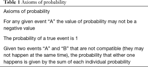
The debate on the definition of probability generated a basic set of axioms that may all reflect the properties of the concept of probability. The entire system of statistical probability is based on these three simple axioms of rules (Table 1) (4).

Table 1 Axioms of probability
Full table

There are also circumstances when information about a certain event may influence the estimate of probability of another event. For example, a physician may think that the probability for a certain disease to occur may be, generally speaking, very low. But, if the patient is exposed to a relevant risk factor for this disease, then the physician’s estimate of probability may change and he may think that the patient is more exposed to this particular disease. In this example, the probability of a certain event is modified after another separate event happens. This is the concept of “conditional probability”. Frequently, a cause-effect relationship between two events may be found under the concept of “conditional probability”.

Distribution of probability

In many situations, the events of interest have a natural interpretation in numerical terms. For example, let’s take into consideration a few typical outcome variables such as diastolic blood pressure, distance walked on a stress test, or the expenses of a family. In all these cases, it is useful to introduce a “random” variable among the results of the real, actual numbers. “Random” or “aleatory” refers to the uncertainty related to the specific value that the variable will receive in a given patient, in a given experiment, at a given time, etc.

In order to express and quantify the uncertainty of the possible values of the aleatory variable, we will introduce the concept of the distribution of probability. This is a mathematical model that is able to link every value of a variable to the probability that this value may be actually observed. Based on the scale used to measure the variable, we may distinguish between two different distributions of probability (5,6):

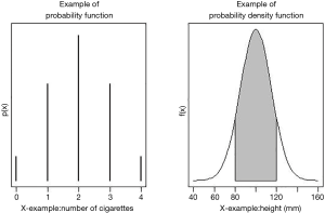
• “Continuous distribution”: the variable is presented on a continuous scale (example: the diastolic blood pressure, a distance, etc.). A distribution of probability of a continuous variable gives a probability to an interval of numbers (Figure 1). The probability that a given value of a variable falls in a specific interval is between 0 and 1. The probability that an interval may include all the possible values is 1.
• “Discrete distributions”: the variable is measured with whole numerical values (for example, number of cigarettes in a period of time). Each probability is a number between 0 and 1. The sum of the probabilities of all the possible values is 1 (Figure 1).

Figure 1 Probability distribution: discrete case and continuous case.

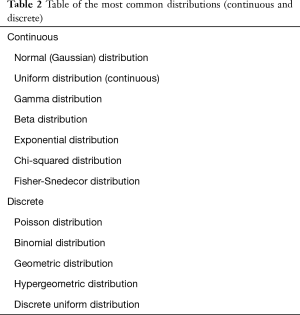
From a formal statistical standpoint, the distributions of probability are expressed by a mathematical formula called “function of density of probability”, called “f(x)” for continuous distributions or “p(x)” for discrete distributions (Figure 1). Table 2 shows the most common continuous and discrete distributions of probability.

Table 2 Table of the most common distributions (continuous and discrete)
Full table

Some theoretical distributions of probability are important because they match very closely the distribution of many variables that may be observed in the real world. Among others, the “normal” distribution is the one that has the most important role in inferential statistics, because many statistical techniques are based on this distribution. The “bell-shaped” curve of the normal distribution is able to describe very well data histograms of variables that are continuous and have a symmetrical distribution. This distribution is frequently used in medicine because many clinical variables may empirically present the typical shape of normal distribution. For example, the linear regression is based on this distribution.

In other cases, the shape of the distribution is not completely normal and there are mathematical transformations that can help the statistician to “normalize” the distribution of data (7).

The importance of the normal distribution should not minimize the role of other types of distribution, because many statistical models have been created in order to bypass the issues of non-normally distributed sets of data using different types of distributions. For example the generalized linear models can assess different types of the outcome distribution such as gamma, binomial, poisson distribution, etc.

Binary variables (dichotomous) are those variables where two only values are allowed to describe a phenomenon, defining two opposite situations (yes or not, alive or dead, etc.). The concept of probability may also apply to these variables, both as an aggregate property ((if a “representative” sample is considered and analyzed, the probability is the rate between the number of outcomes resulting in “yes” and the total number of the subjects of the sample) or an individual probability (the propensity or risk to fall into one specific category). Using this interpretation, probability for categorical variables may be described as well with a value between 0 and 1 and may be analyzed as the dependent variable in an appropriate regression model, for example the logistic regression model (7).

Take home messages

• Uncertainty characterizes every question of inference or decision in clinical research;
• Probability theories provide all the instruments and methodologies to measure these uncertain phenomena. In particular, probability may describe the proportion of times that a certain observation may occur in a large set of observations;
• In statistics, different inferential approaches are based on a probabilistic background: the frequentist (more widely used) and the Bayesan approach;
• The normal distribution has a pivotal role in clinical research because many variables present this type of distribution. Many statistical models are based on this distribution. Many alternatives are available for different type of distributions.

Acknowledgements

None.

Footnote

Conflicts of Interest: The authors have no conflicts of interest to declare.

References

1. Agresti A, Finlay B. Statistical Methods for the Social Science. 4th edition. Upper Saddle River, New Jersey: Prentice Hall, 2009.
2. Pelosi MK, Sandifer TM, Cerchiello P, et al. Introduzione alla Statistica. 2th edition. Napoli: Edizioni Scientifiche Italiane, 2008.
3. Hájek A. Interpretations of Probability. In: Zalta EN, editor. The Stanford Encyclopedia of Philosophy. Stanford, CA: Metaphysics Research Lab, 2012.
4. Grimmett GR, Stirzaker DR. Probability and Random Processes, 3th edition. Oxford: Oxford University Press, 2001.
5. Dall’Aglio G. Calcolo delle probabilità. 3rd edition.Bologna: Zanichelli, 2003.
6. Ross SM. Introduction to probability models. 9th edition. Cambridge, Massachusetts: Academic Press, 2008.
7. Bacchieri A, Della Cioppa G. Fundamentals of Clinical Research. Bridging Medicine, Statistics and Operations. Milan: Springer, 2007.