The use of correlation functions in thoracic surgery research
Introduction
Correlation functions consist of a broad variety of statistical tests, used to describe the relationship between two, or more, sets of data. Those functions, whether they are parametric or non-parametric, are used in medical studies to characterize the strength of this relationship, and the direction of the relationship.
We will successively introduce parametric tests such as the Pearson correlation coefficient, the linear regression model, followed with non-parametric tests such as the Spearman and Kendall rank correlation tests. Finally we will say a few words of calibration, used to evaluate risk scores. The principle of each test will be described and illustrated with selected examples found in medical literature.
Pearson correlation coefficient
Principle
The Pearson product-moment correlation coefficient, more often known as the Pearson Correlation coefficient (also referred to as the Pearson’s r), is a measure of the linear correlation between two variables (1,2).
For two variables x and y, the Pearson correlation coefficient is defined as the covariance of x and y divided by the product of their standard deviations. The Pearson coefficient varies from −1 to +1, where negative values indicate that y decrease with x and positive values indicate that y increase with x. The strength of association between the two variables is considered important (or very strong) if the coefficient ranges from 0.8 to 1, moderate (or strong) from 0.5 to 0.8, weak (or fair) from 0.2 to 0.5, and very weak (or poor) when less than 0.2. When the correlation coefficient is equal to 0, the two variables are independent from one another. When it is equal to 1 they are perfectly correlate in a positive way, whereas when it is equal to −1 the variables are perfectly correlate negatively (anti-correlation).
Mathematically, the correlation coefficient is expressed by the formula:
r= cov xy/√(var x)(var y) = Σ(xi−mx)(yi-my)/ √Σ(xi−mx)2Σ(yi−my)2
Where cov is the covariance, var the variance, and m the standard score of the variable.
For a given value of r and the degrees of freedom of the variables, the correlation table described by Fisher and Yates allows estimation of the risk α.
Selected literature example
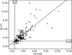
Wu et al. studied the Haller index of their patients on pre-operative CT-scans and chest X-rays, before a Nuss procedure was undertaken (minimally invasive technique of surgical correction of pectus excavatum) (3). For 154 patients, they compared the numerical values of each pair of Haller Index on pre-operative chest X-rays (x) and CT-scan (y), and studied the correlation between the variables with the Pearson’s correlation coefficient, represented on a graph (Figure 1). With a correlation coefficient of 0.757, they concluded that the two chest imaging modalities had a good correlation for the Haller Index pre-operatively.
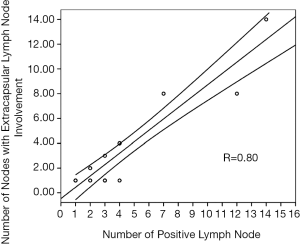
Another example of correlation can be found in the study published by D’journo et al. in 2009 (4). In this study, 94 patients with locally advanced esophageal cancer were included, with lymph node involvement in 32 patients. Metastasis was detected in 120 lymph nodes and extra-capsular extension in 49 lymph nodes. The authors used a Pearson correlation function in the first part of their results to summarize the relationship between the number of nodes with extra-capsular lymph node involvement (y) and number of positive lymph node (x) (Figure 2). They showed a strong, significant, correlation: r=0.8; P=0.01.
Limits
There are limits to the use of the Pearson correlation test. It can only be used for two sets of numerical variables, one set at least with a constant variance. Moreover though the test evaluates the dependence between those variables it does not presume of the causal relationship involved.
Linear regression
Principle
Linear regression is an approach used to characterized the dependence relationship between two variables when one is the direct cause of the other (for example the link between the dose of a drug and the length of survival of a patient), when the modification of value of one variable induces as a direct consequence a modification of the other value, or when the main purpose of the analysis is the prediction of one variable from the other (1,2,5).
For a given n number of pair of two variables x and y, linear regression model can be described with a simple formula:
y = xβ + ε
Where β is the regression coefficient and ε represents the disturbance term or noise.
The regression coefficient can be estimated:
[Σxiyi−(ΣxiΣyi/n)]/[Σxi2×(Σxi)2/n]
Several conditions must be met for an adequate use of linear regressions models. The relationship between the variables must be linear, the predictor variable (x) measurements are considered without error, both variables must have similar variance, and the errors of the response variable (y) must be uncorrelated to each other.
Selected literature example
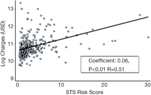
A perfect example of linear regression can be found in the article of Arnaoutakis et al. (6). The authors compared the charges of hospital stay with the Society of Thoracic Surgeon (STS) risk scores during aortic valve replacement. Because the histogram of absolute charges revealed a non-normal distribution, they performed a logarithmic transformation to respect assumptions of linear regression. Furthermore the authors verified the variance of STS risk scores before creating the model. Finally these precautions allowed them to use a regression linear analysis to describe the relationship between log charges (y) and STS risk score (x) during aortic valve replacement (Figure 3). The authors demonstrated a positive correlation between the two variables (correlation coefficient 0.06, 95% CI: 0.05-0.07, P=0.01).
Limits
Linear regression analysis can be used both for univariate or multivariate analysis. But the assumptions needed for its application must be respected. Furthermore the distribution of the variables must be monotonic. For example, if a variable x has a parabolic distribution, the relationship with another variable y if described with a straight line, used for linear regression, will be inadequate.
As with the Pearson correlation coefficient, linear regression analysis does not presume of the causal link between the studied variables.
Non-parametric tests: Spearman and Kendall correlation
Spearman’s rank correlation coefficient
Principle
Spearman’s correlation coefficient can be used to measure the dependent relationship between both continuous and discrete variables, when this relationship is not linear (as opposed to the classic Pearson correlation) (1,2). It can also be used when comparing one continuous variable and one categorical variable.
For two set of variables x and y, each raw scores xi and yi are converted to ranks Xi and Yi. The Pearson correlation coefficient is then used on the ranked variables, following the formula:
ρ = (6Σdi2)/[n(n2−1)]
Where di=Xi−Yi, is the difference between ranks.
The coefficient ρ ranges from −1 to +1, in a similar way as the Pearson correlation coefficient. Accordingly the interpretation of the values is the same as well.
Selected literature example
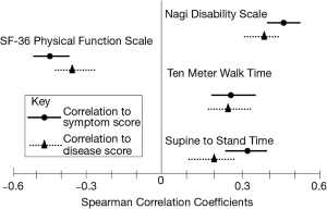
Whitson HE et al., wished to correlate symptom scores with function measures, and with disease scores (7). Each set of data is a set of quantitative variables, each score corresponding to a specific stage, or rank, of the disease concerned. The authors performed correlations between the different scores for several diseases in older adults and summarized the results on a graph (Figure 4). Because of the Spearman correlation, they were able to show the strength of correlation between function measures and symptom scores and disease scores at one glance. The reader can easily evaluate the pertinence of each score scale to estimate symptoms.
Limits
Spearman’s rank correlation coefficient is adequate to describe a monotonic relationship between two variables, but as for the tests previously described, not the causal relationship between them.
It can cause difficulties for the classification of data, a process which might be time-consuming and lead to value duplicates. Spearman’s coefficient should be chosen when the data set is small and the conditions for parametric tests, such as the Pearson correlation coefficient, are not met.
Kendall rank correlation coefficient
Principle
Kendall rank correlation coefficient, also called Kendall’s tau (τ) coefficient, is also used to measure the nonlinear association between two variables (1,2,5). It is used for measured quantities, to evaluate between two sets of data the similarity of the orderings when ranked by each of their quantities.
It can be expressed with the formula:
τ = [(concor)−(discor)]/[0.5n(n−1)]
Where concor is the number of concordant pairs and discor the number of discordant pairs.
The Kendall rank ranges from −1 to +1 and has a similar interpretation as both Pearson and Spearman’s correlation coefficients.
Selected literature example
Sinai CZ studied post-operative high-density lipoprotein cholesterol (HDL-C) levels in children undergoing the Fontan operation (surgical treatment of single ventricule defects) (8). The Kendall rank correlation coefficient was used to correlate The HDL-C levels (baseline and 24-h post-operative) with duration of post-operative chest tube drainage and total hospital length of stay. Though in this case no statistical significance was found.
Another study realized by Wang ZT et al. illustrates the use of the Kendall rank correlation coefficient (9). For 39 patients, the authors used the Kendall correlation to analyze the factors related to the percentage of volume of functional lung receiving ≥20 Gray (FLv20). They showed that the number of non-functional lung had a negative relation with the percentage of FLv20 decrease (r=−0.559, P<0.01), while the distance of planning target volume and non-functional lung center had a positive relation with the percentage of decrease FLv20 (r=0.768, P<0.01).
Limits
The Kendall rank correlation coefficient is used to test the strength of association between to ordinals variables, without presuming of their causal relationship.
Calibration
Principle
Medical studies often use multivariate logistic regression analysis, such as Cox logistic regression, to predict clinical outcomes and create Risk scores. These models are adequate for both categorical and continuous variables, and censored responses as well. Once the model is create, before it is used in a clinical setting, its fit with reality must be evaluated (10). Calibration is defined as the agreement between observed outcomes and predicted probabilities, and is evaluate with goodness of fit tests (5).
Selected literature example
Steyerberg et al., used a multivariate logistic regression analysis to identify criteria linked to 30-day mortality after esophagectomy (11) Based on these results the authors proposed a score to evaluate pre-operatively the surgical mortality of patients with esophageal cancer. In order to assess the performance of this score they studied the calibration of the score with the Hosmer-Lemeshow goodness of fit test (Figure 5). Moreover, in this study, the authors assessed the discrimination of the score. Discrimination refers to the ability to distinguish patients who will die from those who will survive. In this example it was quantified by the area under the receiver operating characteristic curve (AUC). The score evaluate in this study showed a low discrimination but a good calibration.
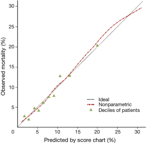
Reproduced from the article of Steyerberg et al. (J Clin Oncology 2006). Calibration of predictions of 30-day mortality after oesophagectomy (n=3,592).
Limits
Calibration has a very specific use and aim. The goodness of fit test chosen depends of the type of explanatory variables previously studied with the logistic regression analysis.
Conclusions
Correlation functions and associated statistical tools such as regression models are widely used in medical studies. Though they each have specifics domains of applications, they share the limit of being unable to evaluate the causal relationship between the studied variables. Basic knowledge of correlation functions is necessary for the clinician, both to perform and understand medical studies.
Acknowledgements
Disclosure: The authors declare no conflict of interest.
References
- Schwartz D. Méthodes statistiques à l'usage des médecins et des biologistes. Médecine-Sciences Flammarion 1963:291.
- Huguier M, Flahaut A. Biostatistiques au quotidien. Paris: Elsevier, 2000:204.
- Wu TH, Huang TW, Hsu HH, et al. Usefulness of chest images for the assessment of pectus excavatum before and after a Nuss repair in adults. Eur J Cardiothorac Surg 2013;43:283-7. [PubMed]
- D'Journo XB, Avaro JP, Michelet P, et al. Extracapsular lymph node involvement is a negative prognostic factor after neoadjuvant chemoradiotherapy in locally advanced esophageal cancer. J Thorac Oncol 2009;4:534-9. [PubMed]
- Agresti A. Categorical Data Analysis. Wiley Series in Probability and Statistics 2013.
- Arnaoutakis GJ, George TJ, Alejo DE, et al. Society of Thoracic Surgeons Risk Score predicts hospital charges and resource use after aortic valve replacement. J Thorac Cardiovasc Surg 2011;142:650-5. [PubMed]
- Whitson HE, Sanders LL, Pieper CF, et al. Correlation between symptoms and function in older adults with comorbidity. J Am Geriatr Soc 2009;57:676-82. [PubMed]
- Zyblewski SC, Argraves WS, Graham EM, et al. Reduction in postoperative high-density lipoprotein cholesterol levels in children undergoing the Fontan operation. Pediatr Cardiol 2012;33:1154-9. [PubMed]
- Wang ZT, Wei LL, Ding XP, et al. Spect-guidance to reduce radioactive dose to functioning lung for stage III non-small cell lung cancer. Asian Pac J Cancer Prev 2013;14:1061-5. [PubMed]
- Harrell FE Jr, Lee KL, Mark DB. Multivariable prognostic models: issues in developing models, evaluating assumptions and adequacy, and measuring and reducing errors. Stat Med 1996;15:361-87. [PubMed]
- Steyerberg EW, Neville BA, Koppert LB, et al. Surgical mortality in patients with esophageal cancer: development and validation of a simple risk score. J Clin Oncol 2006;24:4277-84. [PubMed]


