How to analyze tumor stage data in clinical research

Introduction

The tumor staging system is commonly used to categorize the extent of a malignant disease in a given patient at various time points at or after diagnosis. Tumor staging plays a critical role in optimizing cancer treatment for better patient care. Because of its pivotal function, tumor stage data is inevitably encountered in cancer-related clinical research. In well-designed randomized controlled oncology clinical trials, stage is commonly included as an integrated factor to define the targeted study population, or as a stratification factor in randomization procedure to reduce bias in outcome comparisons between treatment groups. However, there are challenges when analyzing data involving tumor stage in observational studies. For example, when a clinician is reading a recently published research paper examining the survival benefit between two treatments based on data from patients treated in a single institution, he or she might wonder whether the incomparable stage distributions between groups bias the results. Various statistical methods can be used to address this clinician’s concerns. But which method to choose, or just what should one look for to see whether the analysis carried out was actually appropriate, can be overwhelming for oncology researchers without extensive statistical training, probably more so for those who recently joined the field.

Herein, through illustrations of the clinical features and statistical properties of tumor stage data and introductions of statistical terms and methods in specific examples, we hope to increase the awareness of the need to apply proper statistical analytic methods and make scientifically sound interpretations.

Statistical basics—a quick review

Before we dive into examples, a quick review of basic statistical concepts may be helpful for readers to get familiar with the technique aspects of this paper. One common example of analyses in oncology research is to evaluate association between potential risk factors and disease incidence, or between potential prognostic factors and patient outcomes. Statisticians use the term of “variables” to refer to these factors or clinical outcome measures. The variables in the associations to be evaluated are distinguished as either independent (explanatory) or dependent variables. Although it is not strictly accurate, independent variables are commonly thought to be the “predictors” that forecast the results measured by the dependent variables. For example, patients with heavy smoking history (independent variable) have higher risk of developing lung cancer (dependent variable) than those don’t. Or, a new chemotherapy (independent variable) may prolong patients’ overall survival (dependent variable) compared to the standard care treatment.

Different variables considered in any research can carry various statistical properties which is an important aspect for choosing appropriate analytic methods. Statisticians examine the variables starting with their measurement scales, since these scales link to the probability distributions which underline the assumptions of every statistical testing and estimation methods. For example, patient weight, a continuous variable, is commonly considered normally distributed. This normality is one of the key assumptions for the two-sample t-test if one would like to compare patient weight measured at enrollment between two treatment groups in an early stage colon cancer clinical trial. When another variable, number of lymph nodes examined, is to be compared, the two-sample t-test may not be appropriate since the normality assumption may not fit a count variable. In this situation, a test which does not rely on normality assumption such as Wilcoxon Rank Sum test can be considered. Based on measurement scales, variables can be grouped into three statistical types: continuous, count and categorical data. Within categorical variables, variables are further categorized into nominal or ordinal variables. The definition and characteristics of each type of the variable are shown in Table 1. Appropriate statistical methods are determined by a variable’s measurement scale in conjunction of other factors, such as research aims, patient sampling method (e.g., independent vs. clustered vs. matched sampling), sample size, and more.

Table 1 Types of variables in biomedical research
Full table

Tumor staging—a prognostic evidence-based consensus

Presently there are many tumor stage systems, such as the TNM stage system established by the American Joint Committee on Cancer (AJCC) (1), the FIGO stage system established by the International Federation of Gynecology and Obstetrics (FIGO) (2), and the gastric cancer stage system established by the Japanese Gastric Cancer Association (JGCA) (3). In addition, the staging classification can be made by different experts. Clinical staging termed with cT, cN, and cM is commonly determined by clinicians. cTNM is the extent of disease defined by diagnostic study before information is available from surgical resection or initiation of neoadjuvant therapy, within the required time frame (1). When clinical staging is supplemented by findings from surgical resection and histologic examination of the surgically removed tissues by pathologists, the staging results are termed as pTNM. This adds significant additional prognostic information that is more precise than what can be discerned clinically before therapy (1). For the purpose of the discussion, we briefly discuss tumor stage classification and how it was developed, based on the most current version of the AJCC cancer staging manual (1), without distinguish between cTNM and pTNM.

Generally, the anatomic extension of the disease forms the base of the staging systems, including information regarding the primary tumor, regional lymph nodes, and distant metastases. The system uses shorthand notations T, N, and M to describe the stage of a certain cancer:

• T: reflects the size or invading depth of tumor, and whether nearby organs are invaded. Tumor size (commonly in mm) is a continuous variable, whereas the extent of contiguous spreading of primary tumor is a categorical variable. The definition of T stage classification depends on primary tumor location. For example, tumor size is a key factor in breast cancer, whereas the depth of invasion is more prognostic in colorectal cancer.
• N: reflects the presence or absence of involved lymph nodes. Depending on tumor site or location, the number of involved nodes is additionally taken into account for the classification. This data is naturally a binary or a count variable. When the N component itself is a main research factor, the total number of examined lymph nodes sometimes also plays a critical role in the analysis.
• M: reflects the presence or absence of metastases. The metastases commonly present in more than one organ or sites. When overall presented (metastases in at least one organ/site) vs. not presented (no metastases), this data is a dichotomous variable. On the other hand, number of metastatic sites is a count variable. When the research interest is specific to advanced disease stages, the locations of metastases may be taken into the considerations.

These root data were the basis to define individual T, N, and M classifications. These three components were combined into the anatomic stage (also called prognostic) groups. Although details of the classification criteria vary among tumor types, the establishment and refining (i.e., updating) of the stage groups were indeed supported by the prognostic analyses, which evaluated and compared various combinations (i.e., prediction models in statistical language) of anatomic data in relation to survival outcomes or treatment responses through large databases. For instance, the AJCC colorectal staging system was developed based on the National Cancer Data Base and the Surveillance Epidemiology and End Results (SEER) database. For either individual T/N/M or overall stage groups, the increasing values (e.g., T0/1/2/3/4, or stage I/II/III/IV) denote greater extent of cancer and/or increasing prognostic severity of the disease. This fact groups most of the tumor staging related variables into ordinal categorical variables.

In addition to tumor specific T/N/M stage classifications, a different system for designating the extent of disease and prognosis may be applied. For example, the AJCC staging for lymphoma adopted the Ann Arbor classification system (4). Since the 7^th edition, the AJCC staging system also started to formally incorporate fully-validated non-anatomic prognostic factors such as Gleason’s score in early stage prostate cancer. In summary, tumor stage classifications are tumor/histologic type-specific, and the increasing levels of the groups signify the increased prognostic severity of the disease. This in turn provides the basis to classify the overall tumor stage variable to be an ordinal categorical variable (see Table 1).

Analyzing tumor stage data—a state-of-art process

Overview

When tumor staging data are involved, how to choose proper statistical methods and strategies depends on a few important factors. The first essential factor is the research goal of the study. Is the goal to investigate some factors affecting tumor stage (i.e., considered as the dependent variable) or outcomes being affected by tumor stage (i.e., considered as the independent variable)? The second factor is what role, as an independent variable, tumor stage plays in the study. Is tumor stage the main investigational potential predictor of patient outcomes, or is tumor stage a key supplemental factor that may confound or alter the association between the main investigational factor and outcome? The third factor is the depth of tumor stage data to be evaluated in the proposed association study. Is overall stage sufficient to demonstrate the prognostic impacts, or should the heterogeneity in prognostic impacts of the T/N/M stages be assessed separately or should the root data (e.g., continuous tumor size or the count of the involved LNs) be further examined?

To ease the illustration, we will only focus on the overall stage which has four possible levels: Stage I, II, III, and IV. This variable is an ordinal variable with nature order but the exact distances between categories cannot be quantified. As we mentioned previously, the measurement scale of the variables (continuous, count, ordinal, or nominal) is one of the key statistical considerations for choosing the appropriate statistical analysis methods. Therefore, we illustrate statistical methods based on the types of variables other than tumor stage involved in the analysis, when they are nominal, ordinal or continuous variables. Some methods treat the two variables in an association evaluation symmetric, i.e., either one can be considered as dependent or independent variable. Others make clear distinguish between two. These will be explained when it is applicable in the following sections. In addition to introduce the methods for hypothesis testing or parameter estimation, the reasoning of why and how to properly conduct the analyses will be discussed according to the unique situation described in each example.

The examples presented here are not necessarily based on real research data. Using hypothetical data in some cases was intended to demonstrate the key concepts, rather than describe a real research question. A p-value that is less than 0.05 is considered a statistical significant for all the examples. Many excellent texts provide the details required for performing analyses, and data analysis methods included in this paper can be found in a classic categorical data analysis text by Agresti (5) and survival analysis by Miller (6).

Example 1: are the TNM stages comparable among two or more groups?

In a clinical trial, patients diagnosed with lung cancer were randomized to the experimental and control groups. Unfortunately stage was overlooked as one of the stratification factors during the randomization procedure in the design. Therefore, examining whether the stage distribution was comparable between the two groups was necessary, since the treatment effect comparison can be confounded by stage if the disease severity of the experimental and control groups was different. In this example, treatment group is a nominal variable. Number of patients was tabulated in Table 2 by treatment and stage groups. This table is called contingency table in categorical data analyses. For example, among stage I patients, 63% (22/35) and 37% (13/35) patients were randomized onto the experimental and control arms, respectively.

Table 2 Assessing whether the stage distributions are comparable between two treatment groups in a randomized clinical trial (Example 1)
Full table

In practice, Chi-squared test is probably the most common statistical method used for testing independence between two categorical variables in clinical research. In this example, same distributions of stage between two treatment groups imply that the treatment assignment was not dependent on patients’ disease severity classified by tumor stage. The Chi-squared test produced a P value of 0.168 based on data shown in Table 2. One could’ve concluded that there is no statistically significant difference in stage distribution between two groups, i.e., the treatment assignment was not dependent on tumor stage. However, the Chi-squared test does not take account of the nature order in tumor stage variable. By close look at the data tabulated in Table 2, one can see an increasing trend in percent of patients assigned onto the control arm as the tumor stage advances, which is contradict to the conclusion by the Chi-squared test. A research question which is more relevant to tumor stage variable in this example can be re-phrased to whether one of the treatment groups presents higher rank of disease stage than another, i.e., whether the patients with worse (or better) disease conditions were more likely to be assigned on to one of the treatment groups. The Wilcoxon Rank Sum test (also called Mann-Whitney U test) is one of the methods that can address this research question. This test assigns rank scores to each category in stage variable which reflect the nature order and compares the mean ranks between treatment groups. The Wilcoxon Rank Sum test gives a P value of 0.035, which indicates there is statistically significant difference in stage ranking between two groups. This confirms the observation that patients with more advanced disease were more likely to be assigned onto control than experimental treatment group. If this unbalance in tumor stage distribution between groups was not controlled, the treatment effect comparison between two groups can be biased.

The Chi-squared test is considered as a global test, since it tests very general alternative hypotheses, i.e., any type of relationship. The result of the Chi-squared test only conveys the presence or absence of the relationship, but not a specific form of the association, such as, monotonic or linear relationship between two variables. In this example, there is a monotonically increasing relationship between tumor stage and the treatment assignment preference towards control group. When extending the nominal dichotomous variable (i.e., treatment in this example) to a variable with more than two categories (e.g., three treatment groups), the Wilcoxon Rank Sum test can be replaced by the Kruskal-Wallis test.

Example 2: does treatment response vary by stage of disease?

As shown in Table 3 and Figure 1, investigators followed a group of previously treated lung cancer patients, with different stages at initial diagnosis, for tumor response to a second or higher line treatment with a combination of standard care regimen and a newly developed biologic agent. In this case, the response status (i.e., complete or partial tumor response) is the dependent variable and the initial stage is the independent variable. The response status has clear order with responders having better treatment effect than non-responders. In other words, the response status is an ordinal variable. The authors were interested to explore whether the initial diagnosis stages predicts treatment responses.

Table 3 Assessing the impact of stage at initial diagnosis on treatment responses in a previously treated lung cancer population (Example 2)
Full table

Figure 1 Percentage of responders stratified by stage in a previously treated lung cancer population (Example 2).

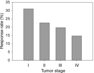
Examining Figure 1 which graphically displays the percentage of responders (i.e., response rate) by stage categories, a monotonically decreasing in response rate is observed as disease stage advances. One of the methods to measure a monotone trend association is estimating Gamma statistics and its associated confidence interval (CI). Gamma statistics ranges from −1 to 1, being closer to either 1 or −1 the stronger the association. However, a significant monotone trend does not necessarily imply a linear trend or other functional forms which require stronger assumptions of the relationship. The Cochran-Armitage trend test was designed to test a linear trend in the probability of either category in a dependent variable (e.g., response rate) according to the values of the independent variable (i.e., disease stage), which is a plausible alternative hypothesis in this example. Table 4 includes the p-values and comparisons when different statistical methods were used. Both Gamma statistics and the Cochran-Armitage trend test demonstrate there is a statistically significant association between disease stage and the response rate, i.e., the response rate decreases as the initial diagnosis stage advances. However, the Chi-squared test fails to detect this association.

Table 4 Comparisons among different statistical tests for testing independence between stage at initial diagnosis and response to treatment in a previously treated lung cancer patient population
Full table

The study in this example was an observational study. Hence, there are likely other factors besides disease stage which can potentially impact the treatment response rate. When these factors are also significantly associated with disease stage, they are called confounders. When only one categorical confounder is considered, the Cochran-Mantel-Haenszel test can be used to test the independence given a particular category of the confounder. This test works better when the association between disease stage and treatment response is similar across categories of the confounder, which can be tested by the Breslow-Day test. However, the logistic regression is a more flexible method which can assess the relationship between disease stage and treatment responses by adjusting for more than one covariate and with less restriction of the statistical measurement scales of the covariates.

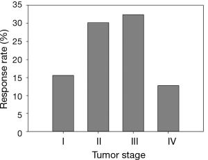
It should be emphasized that all statistical methods require certain assumptions, either liberal or strict. When the assumption is strict, such as the assumption of linear relationship for Cochran-Armitage trend test, the validity of the interpretation of the measure or test depends critically on whether the data meets the required assumptions. Although statistical methods for checking assumptions are beyond the scope of this article, graphically displaying the data can always be explored. As seen in an example modified from Example 2 (Table 5, Figure 2), the linear relationship between two variables is clearly violated—the data exhibits an arch-shaped relationship. A large p-value in the Cochran-Armitage trend test (P=0.322) reflects this violation. Instead, the Chi-squared test detects the dependence of response rate on disease stage with a significant P value (P=0.002). To further evaluate the potential relationship pattern, a univariate logistic regression with disease stage treated as nominal variable shows that the response rate difference lies between stage III and IV patients: the odds of responding to the treatment for stage III patients is 3.274 times greater than that for stage IV patients (odds ratio, 3.274, 95% CI, 1.652 to 6.488, P value, 0.005). The analyze results of different statistical methods and its clinical interpretation were included in Table 6.

Table 5 Assessing the impact of stage at initial diagnosis on treatment responses in a previously treated lung cancer population (modified from Example 2)
Full table

Figure 2 Percentage of responders stratified by stage in a previously treated lung cancer population (modified from Example 2).

Table 6 Comparisons among different statistical tests for testing independence between stage at initial diagnosis and response to treatment in a previously treated lung cancer patient population (modified data from Example 2)
Full table

Example 3: is serum CEA level associated with tumor stages in colorectal cancer patients

Table 7 shows the data of disease stage and carcinoembryonic antigen (CEA) level (a tumor marker) collected at diagnosis. The categorized CEA levels in this example present an ordinal variable with more than two levels. A research question was whether CEA level is associated with tumor stage.

Table 7 Assessing the association between disease stage and carcinoembryonic antigen (CEA) level at diagnosis in colorectal cancer patients (Example 3)
Full table

When both variables are ordinal with more than two levels, Chi-squared test is less likely to be optimal for detecting possible associations. Kruskal-Wallis test can be considered, but it only accounts the ordering in one of the variables. Here, Gamma statistics and other association measures such as Kendall’s Tau are commonly used. Although these measures have close relationship to the Spearman correlation coefficient, they take different values due to very different underlying logic and computational formulas. When data contains many ties, Gamma statistics are preferable. Pearson correlation coefficient may be considered; however, the ordinal variables rarely meet the assumption that two variables follow a bivariate normal distribution. All these association measures are symmetric which means switching of independent and dependent variables will not affect the association estimates. Table 8 listed the method available and its clinical interpretation for this example. The results of all method show that there is a clear positive relationship between two variables.

Table 8 Comparisons among different association measures for assessing the association between disease stage and carcinoembryonic antigen (CEA) level at diagnosis in colorectal cancer patients
Full table

The CEA level variable in this example was actually created by categorizing the continuous CEA variable by chosen cutoffs. When CEA level in a log-transferred form is included in its original form, i.e., a continuous variable, one-way ANOVA is a common method to evaluate the association. Methods, such as ANOVA assumes the continuous dependent variable is normally distributed with constant variance across groups, and the dependent variable is measured independently across the measurement units. ANOVA is a well-developed method which can test general alternative hypotheses, as well as particular association patterns. For example, whether there is a linear increasing trend in log-transferred CEA levels as disease stage advances can be evaluated by a linear contrast in one-way ANOVA, or a quadratic relationship by a quadratic contrast. If normality is not a plausible assumption, e.g., continuous CEA level indeed is highly skewed, one can consider the Kruskal-Wallis test, a nonparametric analogue to ANOVA.

Example 4: is tumor stage the prognostic factor for survival in colorectal patients

In Example 4, a group of newly diagnosed colorectal patients were followed for survival outcome. As described previously, disease stage is a strong prognostic factor of survival outcome by the nature of how the staging was developed. A further question is whether there is any particular association pattern between disease stage and survival. A classic survival outcome, overall survival (OS), is defined as the time from diagnosis date to the date of death due to all causes. By its definition, this is a continuous variable. However the statistical methods for analyzing survival related outcome variables (often called survival analysis) are different from other classic methods for continuous variables (e.g., two-sample t-test, linear regression models, etc.). For instance, the death event in OS may not always be observed for all patients at the time of analysis owing to loss of follow-up or still alive at the end of the follow-up time period. This incompleteness of the data is called censored data. Figure 3 is the most common method to graphically present the data, which is called Kaplan-Meier curve which shows the proportion of patients who were alive at each time point that a death was observed. Log-rank test is a commonly used method to comparing survival outcomes between groups. In this example, there are significant difference in mortality hazards among four stage groups by the log-rank test (P value <0.0001). Like the Chi-squared test, the log-rank test evaluates only the general alternative hypothesis that there exists any type of association between disease stage and OS. Regression type of analysis for survival outcomes is conducted using Cox Proportional Hazard models.

Figure 3 Kaplan-Meier curves of overall survival stratified by disease stage in newly diagnosed colorectal patients. Numbers under the plot are the number of patients at risk at a given time point by stage groups.

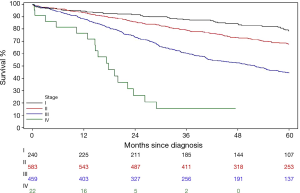
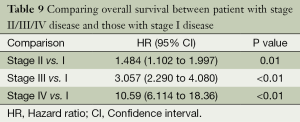
Table 9 presents one way (Model 1) to examine where the differences in OS time lie among stage groups by assigning dummy variables to each level of the stage. When stage I group was considered as the reference group, three dummy variables associated with stage II, III, and IV groups, respectively, were included in the fitted Cox model. Hence, the hazard ratio (HR) was estimated between the pairs of the stage groups listed in Table 9. Consistent with Figure 3, all stage II-IV patients had worse survival time than stage I patients with increased effect sizes (i.e., the values of HRs) as the disease advances.

Table 9 Comparing overall survival between patient with stage II/III/IV disease and those with stage I disease
Full table

Another common practice is fitting a Cox model (Model 2) by including one variable with arbitrary scores assigned to each stage groups, e.g., 1, 2, 3, and 4 for stage I, II, III, and IV, respectively. Here, a linear relationship between disease stage and the mortality hazard is assumed. The linear assumption implies the effect size (i.e., the HR) between consecutive stage groups is the same, i.e., HR comparing stage II to I patients is the same as that comparing stage III to II patients, and so on. Hence the fitted model only gives a single HR and this is actually a very strong assumption. Fitting this model to Example 4 data, the estimated HR is 1.951 with 95% CI of 1.719 to 2.214 and P value of <0.0001. This result indicates there is a statistically linear increasing trend in mortality hazard as disease stage advances, the mortality hazard increased 1.951 times as tumor stage advanced for one incremental level (e.g., advanced from stage I to II, or II to stage III, etc.). Both Model 1 and Model 2 show the mortality hazard is significantly dependent on disease stage. In this case, they are called competing models. Formal model performance comparison can be conducted by Likelihood Ratio test. Here, model performance comparison means whether the simpler model, i.e., Model 2, fits the data better than the more complicated model, i.e., Model 1. The Likelihood Ratio test gives P value of 0.023 (χ², 7.588, df, 2), which rejects the null hypothesis of no difference between two models. Hence, Model 2 fits the data significantly better than Model 1, with the interpretation that the severer initial disease status is correlated to the worse survival with an incremental increasing manner.

Similar to the logistic regression mentioned in Example 1, Cox model can also include more than one covariate for multivariable analyses. A multivariable analysis refers to the situation where more than one predictor is considered to be potentially associated with the outcome (i.e., dependent variable). For example, confounders alter (sometimes mask) the associations between the risk factors and outcomes and they should be adjusted in the multivariable models. Although different types of regression models (e.g., linear, logistic, or Cox model) are used for outcomes with different statistical properties (e.g., normally distributed continuous outcom

Conclusion remarks

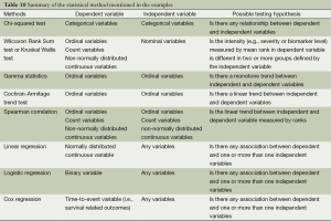
Tumor staging plays a critical role in patient care as well as in oncology research. The ordinal measurement scale of the staging data provided a unique center point for introducing various statistical methods, from categorical data analysis to modeling techniques. The statistical methods mentioned in this article were summarized in Table 10 in pairs of the types of variables which are likely appropriate for the method. However, there are exceptions. Fully examining data in hand is always critical for choosing most appropriate methods.

Table 10 Summary of the statistical method mentioned in the examples
Full table

The concepts illustrated in this article were not intended to be exhaustive, but rather to promote sound statistical analysis thinking. The choice of proper statistical method and analysis strategy depends on the integrated and thorough examination of both clinical research aspects and statistical technologies. The research question is the driving force of study design and data collection, and also sets the basic strategy of statistical analysis. Exploring data by good data presentation, including proper estimates, tabulation and graphing, can positively shape the statistical analysis strategy. Each statistical method was designed for a specific purpose and developed under certain assumptions. Understanding the type of association each method was designed to detect and checking corresponding assumptions are safeguards of the selection of the statistical methods. Hypothesis testing is essential for drawing conclusions, but further analyses should be carried out to characterize the association pattern and quantify the association strength, which are the key components of a proper interpretation of data. Finally, it should be recognized that there is no one size method which can fit every analysis, nor only one method or strategy that can suit a particular research project.

Acknowledgements

Disclosure: The authors declare no conflict of interest.

References

1. Edge SB, Compton CC. The American Joint Committee on Cancer: the 7th edition of the AJCC cancer staging manual and the future of TNM. Ann Surg Oncol 2010;17:1471-4.
2. Pecorelli S. Revised FIGO staging for carcinoma of the vulva, cervix, and endometrium. Int J Gynaecol Obstet 2009;105:103-4. [PubMed]
3. Shimada Y. JGCA (The Japan Gastric Cancer Association). Gastric cancer treatment guidelines. Jpn J Clin Oncol 2004;34:58. [PubMed]
4. Carbone PP, Kaplan HS, Musshoff K, et al. Report of the Committee on Hodgkin's Disease Staging Classification. Cancer Res 1971;31:1860-1. [PubMed]
5. Agresti A. Categorical Data Analysis, 2nd edition. New York: Wiley, 2002.
6. Miller RG. Survival Analysis, New York: John Wiley and Sons, 1981.